

Welcome to another edition of the Hockey Handbook series! In this article I want to equip you with some of the tools you need to grasp “hockey analytics”. I am calling this a primer because we aren’t going to talk about any of the actual metrics classified as analytics, instead we will discuss a couple key introductory concepts and tools for contextualizing the metrics.
Rate Stats
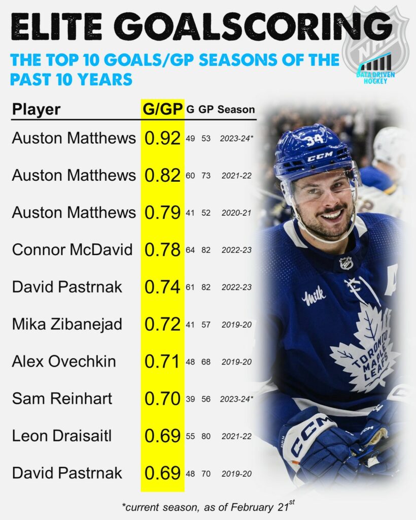
The first concept we will cover is rate stats. What are rate stats? Well, let’s examine this statement: “In the 2021-22 season Auston Matthews scored 60 goals, played in 73 games and was on the ice for a total of 1503.8 minutes.” The 3 stats cited in that statement – Matthews’ totals for goals, games played and time on ice – are NOT rate stats, they are counting stats. All that is needed to collect a counting stat is the ability to count (just count every time Matthews scores and you know how many goals he has). Full disclosure, I just made up that etymology but I’m sticking with it cause it sounds legit.
Why did I act like I was about to explain rate stats but instead explain what counting stats are? For engagement of course. Nah but really, the reason is rate stats are calculated from counting stats. “What came first, the rate stat or the counting stat” is not a rhetorical question, the answer is counting stats. Let’s look at another statement: “In the 2021-22 season Auston Matthews scored at a rate of 0.82 goals per game and 2.39 Goals per 60.” Those are rate stats. Contextualizing a counting stat by dividing by a period of time (such as games played or time on ice) yields a rate stat.
Let’s replace goals with the generic “Stat X” and nail down a formal definition:
“Stat X” per game played (X/GP) and “Stat X” per 60 minutes (X/60) are useful tools for contextualizing counting stats. X/GP normalizes “Stat X” based on the number of games a specific player has played in over the period in question (this can be a single season, a single playoffs, the players career, etc.) and X/60 normalizes “Stat X” based on the specific player’s ice time over the period in question.
It is immediately obvious why this contextualization technique is useful. For example, Auston Matthews has 341 career goals and Phil Kessel has 413. Who is the better goal scorer? If their goal totals were the extent of our information we would have to conclude Kessel is the better scorer. But, we know Matthews has played 531 games in his career and Kessel has played 1286 so we can calculate career goal scoring rates of 0.32 goals/GP for Kessel and 0.64 goals/GP for Matthews. Matthews is clearly the more talented goalscorer of the two.
I know this was a drastic and silly example, but it matters! It’s somewhat surprising how often arguing fans don’t contextualize their data; some unwittingly, but many knowingly, for the purpose of winning an argument via misrepresentation (why bother???? you will always know you’re wrong).
In general, using “per games played” stats facilitates evaluation of players who have played a different amount of games (one of the players may have missed time due to injury, being scratched, etc.). “Per 60 minutes” stats takes us a step further by accounting for differences in ice time between players, even if they have played the same number of games.
Strength States
Strength states describe how many players are on the ice at any given point in the game. For example, the most common strength state is even strength. The game is at even strength when both teams have the same number of players on the ice. Typically this is 5-on-5, but 4-on-4 and 3-on-3 is still considered even strength.
It is useful to sort events (i.e., goals, shots, etc.) by the strength states they occur in because hockey teams perform differently depending on the strength state. For example, the average Goals per 60 minutes rate of teams on the powerplay is much higher than when they are at even strength, which in turn is higher than when the team is on the penalty kill. This makes sense intuitively – with more skaters than your opponent it is easier to maintain possession of the puck and create scoring chances. The following table breaks down average scoring rates by strength state in the NHL this season.
| Strength State | Average Goals For per 60 | Average Goals Against per 60 |
|---|---|---|
| Even Strength | 2.77 | 2.77 |
| Power Play/ Penalty Kill | 7.59 (PP GF/PK GA) | 1.15 (PP GA/PK GF) |
| Empty Net | 7.90 (with EN) | 16.1 (against EN) |
You may be tempted to think that NHL teams should prioritize their special teams and empty net strategies after seeing the above table. After all, the goal scoring rates at those strength states are much higher! However, this is misleading and highlights an important consideration to keep in mind when analyzing rate stats: the timeframe over which the rate is calculated is vitally important! This season NHL teams have played over 44,000 minutes at even strength, just under 9,000 minutes on special teams, and just over 1,000 minutes in empty net situations. Goals per 60 is an excellent stat for highlighting the ease at which NHL teams can score and prevent goals at different strength states but given the large differences in time played at each strength state it is not helpful in determining which strength state is most important. Don’t worry though, we do have a stat for that – goals per game played. Check out the table below.
| Strength State | Average Goals For per GP | Average Goals Against per GP | Percentage of Total Goals per GP |
|---|---|---|---|
| Even Strength | 2.33 | 2.33 | 70% |
| Power Play/ Penalty Kill | 0.65 | 0.098 | 22.5% |
| Empty Net | 0.08 | 0.16 | 7.5% |
70% of goals scored in NHL games this season have come at even strength. This is why even strength is every hockey nerd’s favorite strength state and thus the state upon which most analytics are focused. The other strength states are important, but even strength is the belle of the ball.
Conclusion
In this analytics primer we didn’t directly explore specific metrics, but instead some building blocks necessary to contextualize and assess player statistics effectively.
First we discussed rate stats. By converting counting stats (X) into rates like X/GP and X per 60 minutes we can make meaningful comparisons that account for variations in games played and ice time.
Next, we discussed the significance of strength states. Contextualizing data by considering how many players were on the ice when it was collected is essential for responsible interpretation. We highlighted that 70% of goals are scored at even strength, thus it is the most important strength state.
I hope you enjoyed this analytics primer! Click HERE to browse through other Hockey Handbook entries.
Leave a Reply